Advanced Duct Design: How to size an irregular (polygon) shaped ductwork

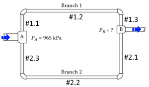
More often than not, engineers have only one choice in the duct geometry design. The only choice left is to design an irregular (polygon) shaped ductwork that will fit within the roof truss configuration as shown in the picture below. Judgement is required for this kind of design application. Do you call it an “integration or innovation” solution to suit available space?

Obviously, one cannot use a conventional ductulator for this kind of duct geometry. So, how to size an irregular (polygon) shaped ductwork like this one?

Fortunately, the fundamental theory of duct sizing allows us to size an irregular shaped duct. For non-circular duct, the hydraulic diameter (Dh) is given by:

It is important to note that the so-called hydraulic diameter (Dh) as expressed is applicable to both circular and non-circular ducts.

For the polygon shaped ductwork as shown in the picture above, the tedious task is to find the cross section area and perimeter of the duct. In terms of design calculations, this accounts for the main difference between an irregular (polygon) shaped duct and a conventional (round, rectangle, oval) duct geometry. At this point of the calculations, it is best to use some design tools (e.g., AutoCAD, polygon calculation software, etc.) that allow you to calculate the cross section area and perimeter of a polygon. This will save you a lot of time.

It is not the intention of this post to illustrate the calculations of duct pressure drop, Reynolds Number and darcy’s friction factor, etc. The formula for duct sizing is documented in the ASHRAE Fundamentals.

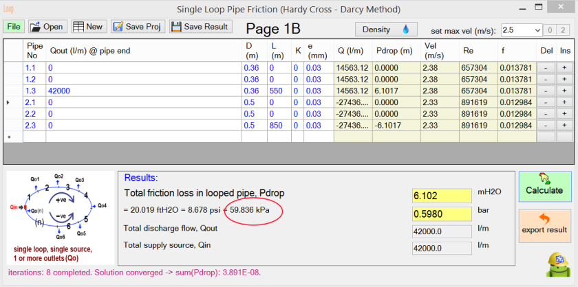
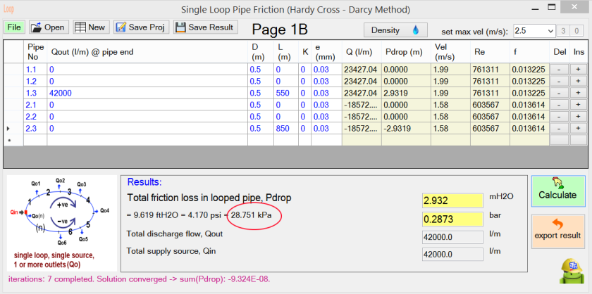
In short, I will use some design tools such as aDuctulator (for Android OS) for duct sizing of any shape as illustrated in the example below.

The following results are obtained using aDuctulator:

(1) Find cross section area and perimeter of the irregular shaped duct.

    

 

(2) Find flowrate or friction loss rate.

    

 

(3) Save/Print results

 

————————————-

 .TT pocketEngineer softDesign

https://sites.google.com/view/pocketengineer

how do I perform my building services engineering calculations faster in a less stressful way?

If you wish to be able to provide answers at anytime, anywhere, or Just-In-Time solutions for your design needs, there are some simple and specially engineered design tool or calculation software that can help you to lessen your unnecessary stress or frustration at work.

Over the years, I have been trying to improve myself constantly on efficiency and productivity aspects of my daily engineering tasks….. still on-going and on-going; lifelong learning! This is trying to move myself towards still-lower and still-competitive cost.

https://sites.google.com/view/pocketengineer

 

Work smart! More often than not, we don’t need complex and complicated design tool to solve simple engineering calculations. The fact is that the result outputs remain as an approximation of reality. Easy to use and knowing its limitations are more important than anything else…. speed counts.

Allow me to borrow the theme of the following question, can you solve it within a minute?

Engineers are taught to tackle problems in the real field in a systematic way, starting from the first principle. So let’s solve the above interesting problem in an engineering way that our lecturers or seniors have taught us.

assign variables: h=hat, d=driver, s=spanner.

derive equations:

eqn(1): h+d=1

eqn(2): d+s=2

eqn(3): h+s=2.4

3 unknown variables, 3 equations, so no need iterations!

from eqn(1): -> d=1-h

from eqn(2) -> d=2-s

so, 1-h=2-s

-> s-h=1 …… eqn(4)

from eqn(3), s=2.4-h

substitute s into eqn(4), -> 2.4-h-h=1

-> 2h=1.4

=>h=0.7 (answer 1) ….horray!

now, continue to find d & s

:

:

:

so, how long did I take??

Gaussian Elimination Method

Engineers like to use Gaussian elimination method for solving systems of linear equations. With the help of computing (apps), solving systems of linear equations become easy. For the above example,  the 3 equations can be re-written to give the following linear system:

1h + 1d + 0s = 1

0h + 1d + 1s = 2

1h + 0d + 1s = 2.4

The augmented matrix is as follows:

(1 1 0 | 1)

(0 1 1 | 2)

(1 0 1 | 2.4)

And the result is shown below:

(1 0 0 | 0.7)

(0 1 0 | 0.3)

(0 0 1 | 1.7)

[solutions: h=0.7, d=0.3, s=1.7]

 

The Egg Basket Problem (Example of Applications in Computing)

Given the amount of complexity in the world today, knowing how to tackle the problem in a simple and faster way is the key to sustain a business. Theoretically, the Egg Basket problem is to be solved using the Chinese Remainder Theorem. However, think like an engineer, I will solve it in an engineering way – simple and efficient! The engineering solution is actually very simple: the iterative approach. As shown in the image below, I have built a Windows program to solve the Egg Basket problem. You can download the Egg Basket solver program (free with no ads, no setup requirement) and try it.

 

————————————-

 .TT pocketEngineer softDesign

https://sites.google.com/view/pocketengineer

 

how-to calculate friction loss (pressure drop) in a single loop (ring main) pipe network

A single loop or ring main pipe network is shown below.

It is a common, reliable and efficient pipe network that engineers would normally adopt in his/her design such as hydrant ring main application, irrigation system, etc.

However, to determine the pressure drop or friction loss in the loop pipe network is not as easy and simple as the one in series pipe network. More often, engineers (count me in) use rule of thumb to estimate the pressure drop as the actual calculation itself (without a computer program) is too tedious and time consuming. The most common and popular method used to calculate the friction loss in a loop pipe network is the Hardy Cross Method (Wiki’s here).

As an engineer, I always think of a simple and effective way to solve a task; explore better methods to do things. In 2015, I spent a lot of time in engineering a program called ePF (easy Pipe Friction) Loop – a simple yet effective solution provider for multi-purpose applications. No pipe network modelling is required. Simple application does not require a complex software to perform the solution. If you need a complex software for your application, you may try EPANET.

Example – Simple analysis of a single loop ring main 

In the loop piping system as shown in the diagram above, the pressure at Node A is 965 kPa, and the total flow rate of water is 0.70 m3/s. Pipe lengths and diameters are as follows:

for branch 1: total pipe length = 550m, diameter = 0.36m

for branch 2: total pipe length = 850m, diameter = 0.50m

The pipe material is Ductile Iron cement-lined pipe. Neglect minor losses, determine the pressure at Node B.

ePF answers:

The snapshot below shows the inputs and results. Note that as only the total pipe length is given for Branch 1, pipe #1.1 and #1.2 are modeled as zero length. Similar for Branch 2.

Given PA = 965 kPa, so PB = 965 – 59.836 = 905.164 kPa

Alternative Design scheme: (reduce pressure drop)

If the pipe diameter in Branch 1 is increased to 0.50m (same diameter as Branch 2), the pressure drop in the looped pipe will reduce by (59.836 – 28.751) = 31.085 kPa (approx. 52%).

Additional Analysis: (motor kW estimation)

Motor kW calculations are done with aPipeSizer (Android version) program.

Assume pump efficiency of 70% and motor efficiency of 85%.

To move the flow with 59.836 kPa head, motor kW required is approx. 70.4 kW.

To move the flow with 28.751 kPa head, motor kW required is approx. 33.8 kW.

Therefore, the motor kW is reduced by 36.6 kW (approx. 52%) in the Alternative Design scheme.

---

Pay & instant Download ePF Loop software via PayPal Digital Goods service:

(Note: To click on “Return to Merchant” button after payment at PayPal page for instant download)

——————————————————————————————————

  .TT pocketEngineer softDesign

how-to obtain curve fitting equation from graph image / published graph (how to get pump curve equation?)

I wanted to obtain curve fitting equation from a graph image / published graph, and I felt powerless to do so. Rethink, Reinvent, I engineered this application – CurveFit Tracer (Windows) primarily for my own use.

This app can help you to achieve a couple of tasks; easy and effective ways.

• to obtain curve fitting equation from graph image/published graph.
• to digitize graph (for further processing in spreadsheet).
• to find complex intersection points of 2 lines.
• to plot pump curves (2 identical pumps in parallel) and system curve.

For example, given the pump curves below, this simple app can trace the existing curve from the graph image/published graph, and obtain a curve fitting equation as shown.

The app can be used as a simple graph digitizer. For example, given the log-log fan curves graph below, the app can extract raw numbers for further processing in spreadsheet.

Graph plotting in Microsoft Excel does not really display intersection point(s) of 2 lines. So along the way, I added a module – Complex Intersections of 2 lines as shown below.

see downloadable intersection point example in applied psychrometric.

And … to plot 2 pumps in parallel curve and system curve.

———————————————————————————————-

Pay & instant download via PayPal Digital Goods service:

(Note: To click on “Return to Merchant” button after payment at PayPal page for instant download)

———————————————————————————————-

 .TT pocketEngineer softDesign